LLM Systems 05: Deep Learning Framework and Auto Differentiation

0. Recap

• Tiling for efficient matrix computation
  • Use shared memory to reduce global memory access
  • Roofline Model & Computational Intensity
• Coalesced memory access
  • Understanding the channel & bank architecture of DRAM
  • Rearrange the thread or data to access global memory in coalesced manner
  • Utilize shared memory to make global memory access coalesced if necessary
  • Avoid bank conflict of shared memory access
    • padding
    • swizzle
• Sparse matrix representation and multiplication
• cuBLAS

1. Learning algorithm for Neural Network

The Learning Problem

使用机器学习解决问题时，首先需要定义一个网络结构，这对应机器学习中假设空间（Hypothesis Space / Model）的概念。如一个简单的 FFN（Feedforward Neural Network）结构如下：

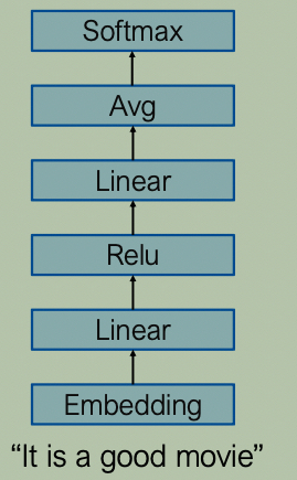
为了让上述网络结构能够解决特定问题，需要对网络进行训练（调整网络的可学习参数以使其能够解决某个问题）。这是一个学习问题，关键要素包括：

• 训练集：给定训练集输入（data）-输出（label）对：\(D=\{ \left( x_{n}, y_{n} \right) \}_{n=1}^{N}\)
  • \(x_{n}\) 与 \(y_{n}\) 都可能是向量。
• 目标：找到模型参数，使模型对每个训练输入产生最准确的输出（或接近的近似）。
• 网络架构已给定，学习的是参数。

Training Loss for Classification

• 交叉熵（Cross entropy）损失：

\[ L(θ)=\frac{1}{N} \sum_{n=1}^{N}{-\log{f(x_{n})_{y_{n}}}} \] - where - \(x_n\)：第 \(n\) 个样本的输入特征 - \(y_n\)：第 \(n\) 个样本的真实类别标签（整数索引，如 0/1/2/…） - \(f(x_n)\)：模型对输入 \(x_n\) 的预测输出向量（通常为 logits 或经过 softmax 的概率） - \(f(x_n)_{y_n}\)：预测向量中，真实类别 \(y_n\) 对应的那个分量，即模型预测为真实类别的概率（或得分） - 直观理解：模型预测真实类别的概率 \(f(x_n)_{y_n}\) 越接近 1，\(-\log\) 越接近 0，损失越小；越接近 0，损失越大（惩罚越重）。

• PyTorch CrossEntropyLoss 的行为：

  • 接收未归一化的 logits（不是概率），内部等价于 log_softmax + nll_loss。

  • 即： \[ \text{CrossEntropyLoss}(z, y) = -\log \left( \frac{\exp(z_y)}{\sum_j \exp(z_j)} \right) \] ​ 其中 \(z\) 是 logits，\(y\) 是真实类别索引。

  • 它不是先算 softmax 再取 log，而是将两步融合，在数值上更稳定（避免 \(\log(0)\) 或指数溢出）。

PyTorch 示例代码：

loss = nn.CrossEntropyLoss()

output = loss(input_logits, target_labels)

grads = output.backward()

本讲要回答的问题：

• how is backward implemented?
• how does it work on any network?

Optimization method of neural networks

Generic Iterative Learning Algorithm

• 问题定义：考虑一个通用的函数最小化问题。
  • 未知变量：\(x\)
  • 目标函数：\(f: \mathbb{R}^d \to \mathbb{R}\)
  • 优化目标： \[ \min_x f(x) \]
• 迭代更新算法：
  • 通过迭代的方式，逐步更新 \(x\)： \[ x_{t+1} \leftarrow x_t + \Delta \]
  • 目标是使得更新后的函数值显著下降： \[ f(x_{t+1}) \ll f(x_t) \]
  • 核心问题：如何找到最优的更新量 \(\Delta\)？

Gradient Descent

• 一阶泰勒展开：对函数在 \(x_t\) 处进行一阶近似： \[ f(x_t + \Delta x) \approx f(x_t) + \Delta x^T \nabla f|_{x_t} \]
• 寻找下降方向：
  • 为了让 \(f(x_t + \Delta x)\) 尽可能变小，需要使 \(\Delta x^T \nabla f|_{x_t}\) 最小。
  • 根据向量内积的性质，\(\Delta x\) 应当取梯度的反方向： \[ \Delta x = -\nabla f|_{x_t} \]
• 参数更新规则： \[ x_{t+1} = x_t - \eta \nabla f|_{x_t} \]
• 超参数：\(\eta\) 是学习率（learning rate），用于控制每次更新的步长。

(Stochastic) Gradient Descent

• 前置设置：设定学习率： eta。
• 初始化：设置初始参数 \(\theta \leftarrow \theta_0\)。
• 训练循环：
  • 外层循环：for epoch = 1 to maxEpoch or until converg
  • 批次循环：for each batch in the data
    1. 初始化总梯度：total_g = 0
    2. 样本循环：for each data (x, y) in data batch
       • 计算误差：err(f(x; θ) - y)
       • 计算当前样本梯度：\(g = \frac{\partial \text{err}(\theta)}{\partial \theta}\)
       • 累加梯度：total_g += g
    3. 批次更新：\(\theta = \theta - \eta \cdot \text{total\_g} / N\) （其中 \(N\) 为当前 batch 的大小）

如何在“任意网络”中计算所有参数的梯度？

• 核心目标：计算损失函数 \(l\) 对每一个网络参数 \(w_i\) 的偏导数： \[ \frac{\partial l}{\partial w_i} \]
• 两大支柱：
  • 前向计算（Forward computation）：从输入层开始，逐层计算网络输出，并最终计算损失。
  • 反向传播（Backpropagation）：从损失开始，利用链式法则，反向逐层计算梯度。
    • 计算图
    • 自动求导

2. Computation Graph

• 神经网络计算过程可以用计算图表示。

• 每个节点表示一个变量或者操作。

• 有向边连接节点，表示操作的输入值。

• 例子：

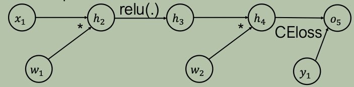
• \(x_{1}\) ：输入

• \(w_{1,2}\) ：模型参数/权重

• \(h_{2,3,4}\) ：中间计算结果

• \(y_{1}\) ：label

• \(o_{5}\) ：输出（loss scalar）

计算过程示例：

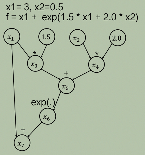
为了执行计算，需要： - 对所有节点进行拓扑排序。 - 给定输入，计算每个节点的值。

拓扑排序：

• 将所有节点放入未处理队列。
• 重复：
  • 找到一个没有未处理入边（入度为 0）的节点。
  • 根据操作计算其值。
  • 将该节点移出队列，加入已处理队列。

3. Auto Differentiation

反向传播

前面已经介绍：为了优化（学习）一个神经网络，需要计算损失函数关于所有网络参数（权重）的梯度。在计算图中，参数也表示为节点（通常为叶子节点）。 - 问题：如何根据计算图计算参数梯度： - 基础：链式法则 -> 反向传播 \[ \frac{dy(z)}{dx} = \frac{dy(z)}{dz} \cdot \frac{dz}{dx} \] 补充说明：关于 \(y(z)\) 符号的理解

• 为什么不写成 \(y(x)\)？ 因为 \(y\) 和 \(x\) 在计算图中不直接相连，中间隔着节点 \(z\)。写成 \(y(x)\) 会抹杀中间变量的存在。
• 为什么不写成 \(y(z(x))\)？ 数学上最严谨，但深度学习框架采用局部视角：每个节点只关心它的直接输入（如节点 \(y\) 只知道输入是 \(z\)）。写成 \(y(z)\) 是为了强调局部梯度 \(\frac{dy}{dz}\)，方便反向传播时按“上游梯度 × 局部梯度”逐层传递。
• 更常见的写法：通常省略自变量，直接写 \(\frac{dy}{dx} = \frac{dy}{dz} \cdot \frac{dz}{dx}\)，像分数约分一样，纯粹表达导数的传递关系。

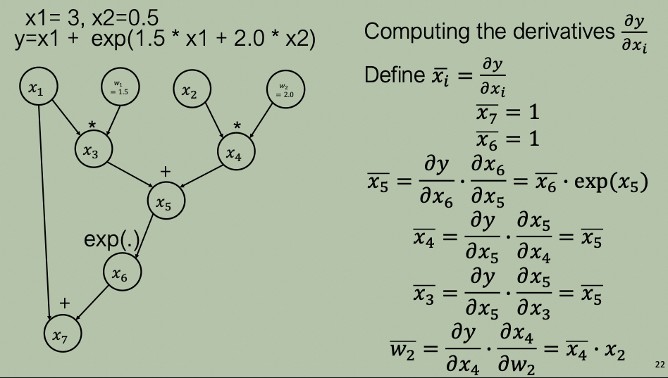
根据计算图进行反向传播计算梯度例子：

对于有多个出度的节点反向传播规则：

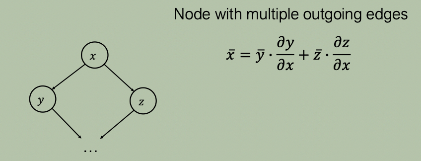
• 节点 \(x\) 参与了节点 \(y\) 和 \(x\) 的计算（输入）
• 反向传播规则（不同节点来源梯度累加即可）： \[ \bar{x} = \bar{y} \cdot \frac{\partial y}{\partial x} + \bar{z} \cdot \frac{\partial z}{\partial x} \]

向量偏导

• 雅可比矩阵（Jacobian Matrix）
  • 对于向量函数 \(y = f(x)\)，其偏导数构成雅可比矩阵： \[ J = \frac{\partial y}{\partial x} = \begin{pmatrix} \frac{\partial y_1}{\partial x_1} & \frac{\partial y_1}{\partial x_2} \\ \frac{\partial y_2}{\partial x_1} & \frac{\partial y_2}{\partial x_2} \end{pmatrix} \]
  • 行：保持 \(y\) 的索引，遍历 \(x\) 的索引（\(J_{ij} = \frac{\partial y_i}{\partial x_j}\)）。
  • 列：保持 \(x\) 的索引，遍历 \(y\) 的索引。

向量-雅可比乘积（Vector-Jacobian Product, VJP）

• 定义：在计算图反向传播中，每个节点接收上游梯度 \(\bar{y}\)，并需要计算传递给下游（更靠近输入）的梯度 \(\bar{x}\)。

  • 上游梯度：\(\bar{y} = \frac{\partial L}{\partial y}\)
  • 下游梯度：\(\bar{x} = \frac{\partial L}{\partial x}\)
  • 数学关系： \[ \bar{x} = J^T \bar{y}, \quad \text{其中 } J = \frac{\partial y}{\partial x} \]

• 推导（链式法则）： \[ \bar{x} = \frac{\partial L}{\partial x} = \left( \frac{\partial y}{\partial x} \right)^T \frac{\partial L}{\partial y} = J^T \bar{y} \]

• 关键理解：为什么不显式构建 \(J\)？

  • 数学上，\(J\) 是 \(y\) 对 \(x\) 的雅可比矩阵，形状为 \(\dim(y) \times \dim(x)\)。在深度网络中，这个矩阵可能极其巨大（例如 \(10000 \times 10000\)），且大多数元素为 0 或具有特殊结构（如对角阵）。
  • 自动微分框架从不真正在内存中创建 \(J\)，而是为每个算子直接定义“给定 \(\bar{y}\)，如何直接算出 \(\bar{x}\)”的规则（即 VJP 规则）。
  • 例如：
    • \(y = Wx\)：VJP 规则是 \(\bar{x} = W^T \bar{y}\)（这里 \(J = W\)，但 \(W\) 本来就存在，无需额外构造 \(J\)）。
    • \(y = \exp(x)\)：VJP 规则是 \(\bar{x} = \exp(x) \odot \bar{y}\)（若显式构建 \(J\)，会得到巨大的对角矩阵，极其浪费）。
    • \(y = \text{ReLU}(x)\)：VJP 规则是 \(\bar{x} = \mathbb{1}[x>0] \odot \bar{y}\)。

• 反向传播 = 计算图 + 链式法则 + 逐节点 VJP

  • 反向传播从损失 \(L\) 开始，沿计算图逆拓扑序遍历每个节点。
  • 每到达一个节点，就调用该节点的 VJP 规则，将上游梯度 \(\bar{y}\) 转换为下游梯度 \(\bar{x}\)，并继续向前传递。

• 总结：VJP 是链式法则在单个节点上的数学表达；反向传播是沿计算图反复应用 VJP；框架只实现每个算子的 VJP 规则，不显式构造雅可比矩阵 J。

• 示例：线性层

  • 前向：\(y = Wx\)
  • 雅可比：\(J = \frac{\partial y}{\partial x} = W\)
  • 反向（VJP）：\(\bar{x} = J^T \bar{y} = W^T \bar{y}\)
  • 结论：在反向传播中，梯度通过权重矩阵的转置进行传递。

反向传播自动求导示意图：

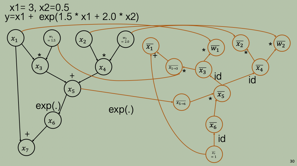
1. 左侧：前向计算图（Forward Pass，黑色部分）

• 目标：从输入计算到最终的标量输出（Loss）。
• 节点与计算：
  • 输入：\(x_1 = 3\), \(x_2 = 0.5\)
  • 权重/常量：\(w_1 = 1.5\), \(w_2 = 2.0\)
  • 中间计算：\(x_3 = x_1 \cdot w_1\), \(x_4 = x_2 \cdot w_2\), \(x_5 = x_3 + x_4\), \(x_6 = \exp(x_5)\), \(x_7 = x_1 + x_6\)。
  • 最终输出 \(x_7\) 即为 \(y\)。
• 方向：数据从左向右、从下向上流动。

2. 右侧：反向计算图（Backward Pass，橙色部分）

• 本质：这就是前向图对应的梯度计算图。它沿着与前向图相反的方向，从最终输出反向传递梯度。
• 起点（右下角）：\(\bar{x}_7 = 1\)。因为 \(\bar{x}_7 = \frac{\partial y}{\partial x_7} = 1\)，梯度从 1 开始传递。
• 边的含义（局部梯度 / VJP 规则）：
  • id：恒等映射，表示梯度乘以 1，直接传递。
  • *：表示乘以常数（如 \(w_1, w_2\)）或另一个输入变量（如 \(x_1, x_2\)），对应乘法节点的 VJP。
  • exp(.)：对应 \(\exp\) 节点的 VJP，梯度乘以 \(\exp(x_5)\)（即前向计算出的 \(x_6\)）。
  • +：对应加法节点的 VJP，梯度直接分发（多条路径求和）。
• 多路径累加（左上方）：
  • 输入 \(x_1\) 在前向图中影响了两条路径：直接传给 \(x_7\)，以及通过 \(x_3\) 传给 \(x_5\)。
  • 因此，在反向图中，\(\bar{x}_1\) 从两条路径接收梯度：一条是 id（来自 \(\bar{x}_7\)），另一条是 \(\bar{x}_3 \cdot w_1\)。两者在 \(\bar{x}_1\) 处通过一个 + 节点累加。
• 权重梯度计算：
  • \(\bar{w}_1 = \bar{x}_3 \cdot x_1\)（上游梯度乘以该权重在前向计算中所乘的输入值）
  • \(\bar{w}_2 = \bar{x}_4 \cdot x_2\)

Implementation

Implementing Backward Pass

def backward_pass(g, end_node):
    """Backpropagation.
    
    Traverse computation graph backwards in topological order from the end node.
    For each node, compute local gradient contribution and accumulate.
    """
    outgrads = {end_node: g}
    for node in toposort(end_node):
        outgrad = outgrads.pop(node)
        fun, value, args, kwargs, argnums = node.recipe
        for argnum, parent in zip(argnums, node.parents):
            # Lookup vector-Jacobian product (gradient) function for this function/argument.
            vjp = primitive_vjps[fun][argnum]
            
            # Compute vector-Jacobian product (gradient) contribution due to
            # parent node's use in this function.
            parent_grad = vjp(outgrad, value, *args, **kwargs)
            
            # Save vector-Jacobian product (gradient) for upstream nodes.
            # Sum contributions with all others also using parent's output.
            outgrads[parent] = add_outgrads(outgrads.get(parent), parent_grad)
    return outgrad

def add_outgrads(prev_g, g):
    """Add gradient contributions together."""
    if prev_g is None:
        return g
    return prev_g + g

代码解释：

• 核心思想：逆拓扑序遍历计算图，逐节点应用链式法则（VJP）。
• outgrads 字典：存储每个节点当前累积的上游梯度。初始只有末端节点（Loss）的梯度 g（通常为 1）。
• 拓扑排序 toposort(end_node)：保证处理某个节点时，所有需要用到它梯度的下游节点都已经计算完毕。
• node.recipe 与 VJP 查找：每个节点记录了自己的前向操作（fun）、前向输出值（value）、输入参数等。框架通过 primitive_vjps[fun][argnum] 直接取出对应的局部梯度计算规则（VJP），完全避开雅可比矩阵的显式构建。
• add_outgrads（多路径梯度累加）：如果一个节点被多次使用（分叉），它的梯度会从多条路径传来。必须通过这个函数将各路梯度相加，对应数学上的 \(\bar{x} = \sum \bar{y_i} \cdot \frac{\partial y_i}{\partial x}\)。

Build the AutoDiff Graph

def make_vjp(fun, x):
    """Make function for vector-Jacobian product.
    
    Args:
        fun: single-arg function. Jacobian derived from this.
        x: ndarray. Point to differentiate about.
    Returns:
        vjp: single-arg function. vector -> vector-Jacobian[fun, x] product
        end_value: end_value = fun(start_node)
    """
    start_node = Node.new_root()
    end_value, end_node = trace(start_node, fun, x)
    if end_node is None:
        def vjp(g):
            return np.zeros_like(x)
    else:
        def vjp(g):
            return backward_pass(g, end_node)
    return vjp, end_value


def grad(fun, argnum=0):
    """Constructs gradient function.
    
    Given a function fun(x), returns a function fun'(x) that returns the
    gradient of fun(x) wrt x.
    """
    def gradfun(*args, **kwargs):
        # Replace args[argnum] with x. Define a single-argument function to
        # compute derivative wrt.
        unary_fun = lambda x: fun(*subval(args, argnum, x), **kwargs)
        
        # Construct vector-Jacobian product
        vjp, ans = make_vjp(unary_fun, args[argnum])
        return vjp(np.ones_like(ans))
    return gradfun

代码解释：

• make_vjp（图构建与追踪）：
  • Node.new_root() + trace(...)：这是自动微分的“录播”机制。它执行一次前向计算，同时把所有的运算步骤和依赖关系记录成计算图（Computation Graph）。
  • 返回的闭包 vjp(g)：封装了反向传播过程。当传入上游梯度 g 时，它会沿着记录好的图调用 backward_pass。
• grad（用户 API 封装）：
  • 为什么需要 unary_fun？因为 make_vjp 只接受单变量函数。subval 把多参数函数中的第 argnum 个参数替换成变量 x，其余参数固定，从而化多为单。
  • vjp(np.ones_like(ans))：反向传播的初始梯度。对于标量损失，其自身的导数为 1；对于向量输出，用全 1 向量作为起始梯度，相当于求其所有输出分量的和（即 \(\frac{\partial \sum y_i}{\partial x}\)）。

Use AutoGrad

# Define training objective
def objective(params, iter):
    idx = batch_indices(iter)
    return -log_posterior(params, train_images[idx], train_labels[idx], L2_reg)

# Get gradient of objective using autograd.
objective_grad = grad(objective)

def neural_net_predict(params, inputs):
    """Implements a deep neural network for classification.
    params is a list of (weights, bias) tuples.
    inputs is an (N x D) matrix.
    returns normalized class log-probabilities."""
    for W, b in params:
        outputs = np.dot(inputs, W) + b
        inputs = np.tanh(outputs)
    return outputs - logsumexp(outputs, axis=1, keepdims=True)

def log_posterior(params, inputs, targets, L2_reg):
    log_prior = -L2_reg * L2_norm(params)
    log_lik = np.sum(neural_net_predict(params, inputs) * targets)
    return log_prior + log_lik

代码解释：

• 前向模型 neural_net_predict：纯 NumPy 实现的多层感知机。核心逻辑是循环执行 outputs = np.dot(inputs, W) + b 然后接 np.tanh 激活。最后使用 logsumexp 做稳定归一化，输出对数概率。
• 损失函数 log_posterior：损失分为两部分。log_prior 是 L2 正则化项；log_lik 是对数似然（np.sum(预测值 * 真实标签)）。两者相加构成后验对数概率。
• 目标函数与自动微分：objective 包装了 log_posterior 并加上负号（因为优化器通常做最小化）。objective_grad = grad(objective) 直接产生一个梯度计算函数。用户无需手动推导任何梯度公式，框架自动完成了反向图的构建与 VJP 调用。
• 实操要点：在训练循环中，直接调用 objective_grad(params, iter) 就能拿到对应参数的梯度，传给优化器（如 SGD、Adam）即可完成参数更新。

How to check the correctness of gradient

• 核心方法：使用有限差分（Finite Differences）来验证梯度计算的正确性。
• 计算公式（中心差分法）： \[ \frac{\partial f(x_1, x_2)}{\partial x_1} = \frac{f(x_1 + h, x_2) - f(x_1 - h, x_2)}{2h} \]
  • 通过计算函数在 \(x_1 + h\) 和 \(x_1 - h\) 处的值，来近似 \(x_1\) 处的导数。
  • 中心差分比前向差分（\(f(x+h) - f(x)\)）的误差更小（误差为 \(O(h^2)\) 而不是 \(O(h)\)）。
• 注意事项（精度控制）：
  • 使用双精度（fp64）：浮点数在计算微小的 \(h\) 时容易产生舍入误差（Catastrophic Cancellation）。如果使用 fp32，分子上的差值可能因为精度不足而变成 0。
  • 选择较小的 \(h = 0.000001\)（即 \(10^{-6}\)）：
    • \(h\) 太大：截断误差大，近似不准。
    • \(h\) 太小：浮点舍入误差大，导致分母虽然小，但分子因精度丢失变成 0，结果为 NaN 或 Inf。
  • 通过图计算两次前向差分：意味着要调用 f(x_1 + h, x_2) 和 f(x_1 - h, x_2) 各一次，总共两次前向传播（Forward Pass）。这也是为什么它常用于小规模网络的调试，因为计算开销是普通前向的 2 倍。

4. Put Together: Implementing a Deep Learning Framework

Deep Learning Frameworks (also for LLMs)

深度学习框架需要具备的能力：

• expressive to specify any neural networks
  • support future custom operators/layers
• productive for ML engineers
  • hide low-level details (no need to write CUDA)
  • automatic differentiation (no need to derive gradient calculation manually)
• efficient in large-scale training and inference
  • automatically scale to data and model size
  • automatic hardware acceleration

典型框架特点：

Aspect	PyTorch	TensorFlow	JAX	NumPy
Primary Use	Deep learning	Deep learning	numerical and ML computing	numerical computing
Programming Paradigm	Dynamic (eager execution)	Static (Graph mode, or Eager)	Functional transformations	Procedural
Autograd	dynamic comp graph	static comp graph	Functional-based with grad/jit	Not available
Hardware Support	CPU, GPU, TPU	CPU, GPU, TPU	CPU, GPU, TPU	CPU only
Ease of Use	Pythonic	a bit learning curve	Pythonic and functional	Very easy, native python
Ecosystem	PyTorch Lightning, TorchVision	TensorBoard, TensorFlow Extended	integrates with NumPy	NA
Parallelism	Multi-GPU with DataParallel or DDP	Multi-GPU/TPU via tf.distribute	Multi-GPU/TPU via pmap	No parallelism

深度学习框架设计原则：

• Dataflow graphs (computation graph) of primitive operators
• Deferred execution (two phases)
  • Define program i.e., symbolic dataflow graph w/ placeholders, essentially constructing the computation graph
  • Executes optimized version of program on set of available devices

基本组成部分（以 TensorFlow 为例）：

• A Computation Graph, which contains these nodes
  • Placeholder: to store the input data (as tensors/multi-dim array)
  • Variable: to store the network parameters
  • Constant: some static data
  • Operation: the mathmatical operations for each neural network layer, the input are any of these nodes, result is stored in output
    • each operation needs to define forward and backward operation
• Session: execution environment
  • Perform computation via the topological sort of the nodes

TensorFlow

TensorFlow v1 采用 声明式编程（静态图）与延迟执行的设计范式，核心是把神经网络训练抽象成一张有向无环计算图（DAG）。

1. 计算图核心示例

以最简单的神经网络层为例： \[ h = \text{ReLU}(Wx + b) \]

在 TensorFlow v1 中，这行公式会被构建为一张包含不同节点的计算图：

import tensorflow as tf

# 定义参数节点 (Variable)
b = tf.Variable(tf.zeros((100,)))
W = tf.Variable(tf.random_uniform((784, 100), -1, 1))

# 定义输入节点 (Placeholder)
x = tf.placeholder(tf.float32, (1, 784))

# 定义操作节点 (Operation) 并构建计算图
h = tf.nn.relu(tf.matmul(x, W) + b)

2. 三类核心节点类型

① Placeholder（输入节点） - 作用：代表输入数据、标签等外部数据。 - 特点：在构建图时不需要赋值，其具体的值在执行时（Execution time）通过 feed_dict 喂入。 - 注意**：TensorFlow v2 中已经不需要显式定义 Placeholder。

② Variable（参数节点） - 作用：代表模型的权重参数。 - 特点：是有状态节点（Stateful nodes）。它们在多次执行图的过程中，会保留当前的值（State is retained across multiple executions）。 - API：tf.Variable(initial_value=None, trainable=None, name=None)。trainable=True 的标志意味着它会被优化器更新。

③ Operation（计算节点） - 作用：定义具体的数学运算，输入是任意其他节点，输出是计算结果。 - 常见 API： - tf.linalg.matmul(a, b)：矩阵乘法（对应 PyTorch 的 torch.matmul）。 - tf.math.add(a, b)：逐元素加法（对应 torch.add）。 - tf.nn.relu(a)：逐元素 ReLU 激活（对应 torch.nn.ReLU）。公式为：\(\text{ReLU}(x) = \max(0, x)\)。

3. 自定义 Operation 节点

要自定义一个算子，需要继承 Operation 基类，并在 __init__ 中传入输入节点，同时实现 forward（前向计算）和 backward（反向梯度计算）函数。

class AddOperation(Operation):
    # 定义加法操作 a+b
    def __init__(self, a, b):
        # a, b 是输入节点
        super().__init__([a, b])

    def forward(self, a, b):  # 计算操作结果
        return a + b

    def backward(self, upstream_grad):
        # ... 定义梯度反向传播逻辑
        ...

4. 定义 Loss 为节点

• 使用 Placeholder 表示真实标签。
• 结合神经网络输出（预测值）和标签节点，构建 Loss 节点。

prediction = tf.nn.softmax(...)  # 神经网络输出
label = tf.placeholder(tf.float32, [100, 10])  # 标签

# 交叉熵损失节点
cross_entropy = -tf.reduce_sum(label * tf.log(prediction), axis=1)

5. 梯度计算与优化器

在 TensorFlow v1 中，梯度计算也是计算图的一部分。

train_step = tf.train.GradientDescentOptimizer(0.5).minimize(cross_entropy)

• tf.train.GradientDescentOptimizer 是一个优化器对象。
• GradientDescentOptimizer(lr).minimize(cross_entropy) 的作用是向计算图中添加优化操作（包括计算梯度和更新参数）。
• 自动微分：TensorFlow 图中的节点自带附件的梯度操作（Attached gradient operations），框架会自动根据计算图进行反向传播（Automatic Differentiation），用户无需手写梯度公式。
• 当 Session 执行 train_step 时，就会自动完成一次前向 + 反向 + 参数更新。

6. 执行机制：Session与两阶段

静态图的“延迟执行”（Deferred Execution）将整个流程分为两个阶段： - Phase 1：定义程序（Define）：构建符号数据流图，不进行实际计算。 - Phase 2：执行程序（Execute）：在可用设备集（如 CPU、GPU）上执行优化后的图。

Session 正是连接这两个阶段的桥梁：它绑定特定的执行上下文（例如 CPU 或 GPU），负责分配资源并运行图。

代码示例（两阶段完整流程）：

import tensorflow as tf

with tf.Session() as sess:
    # Phase 1: Constructing the graph
    a = tf.constant(15, name="a")
    b = tf.constant(5, name="b")
    prod = tf.multiply(a, b, name="Multiply")
    sum = tf.add(a, b, name="Add")
    res = tf.divide(prod, sum, name="Divide")

    # Phase 2: Running the session
    out = sess.run(res)
    print(out)

5. Summary

• Learning parameters of an NN needs gradient calculation
• Computation Graph
  • to perform computation: topological traversal along the DAG
• Auto Differentiation
  • building backward computation graph for gradient calculation
• Put together: Deep Learning Framework
  • Define program i.e., symbolic computation graph w/placeholders/variable/operation nodes
  • Executes (optimized) computation graph on a set of available devices