LLM Systems 10 & 11: Accelerating Transformer Training and Inference

0. Recap

Transformer Architecture：

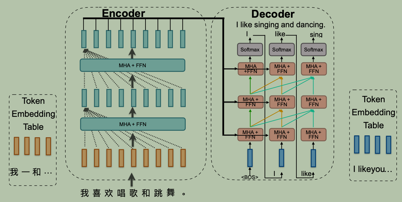
1. Accelerated GPU Computation for Transformer Training

Overview:

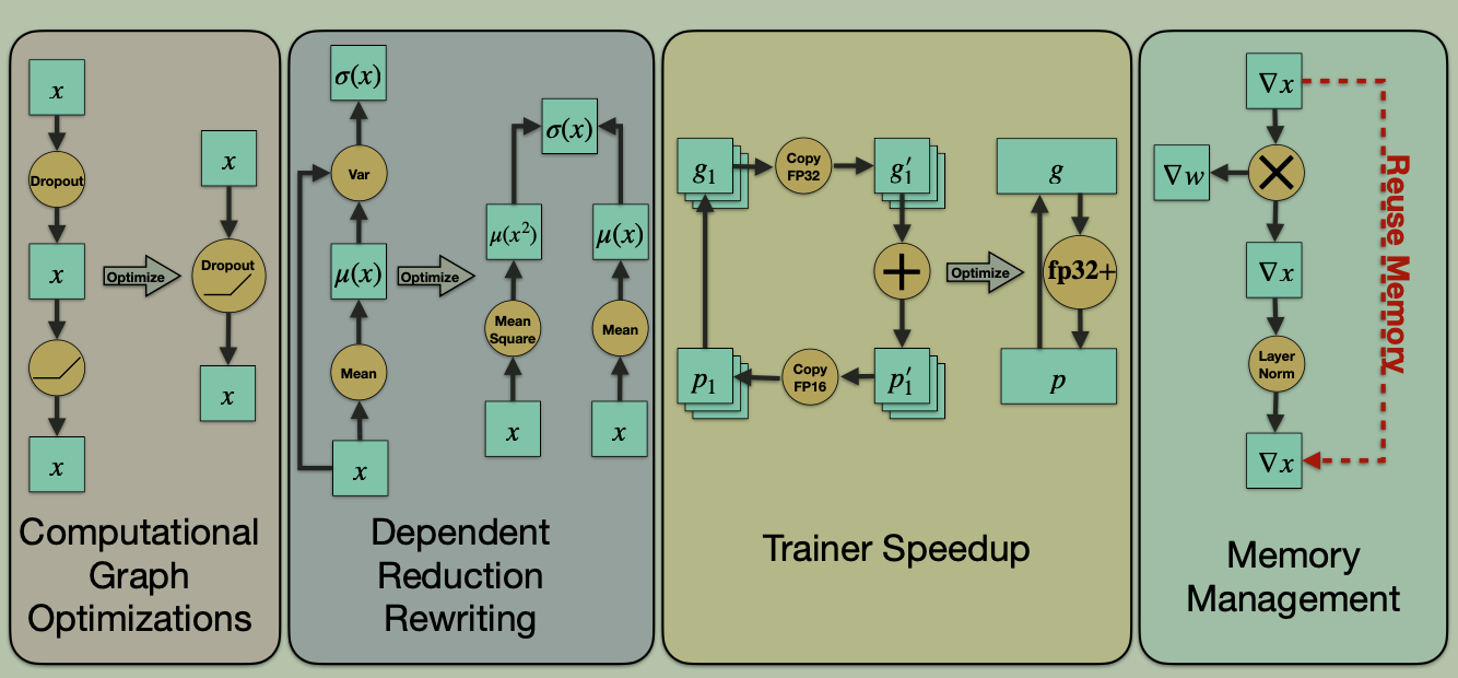
对应下面将要介绍的 4 个优化手段：

• Kernel Fusion：计算图级别优化，通过算子融合减少计算图节点。
• Reduce synchronization：算子内优化，通过算子实现形式变换，减少 kernel 内同步开销。
• Mixed-precision Calculation：框架层面优化，混合精度训练提升训练速度，降低显存开销。
• Memory reuse：细粒度内存管理优化。

1.1 Kernel Fusion

Kernel Fusion Motivation

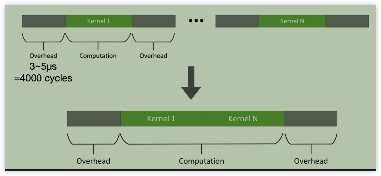
• 将多个小 kernel 融合为一个。
• 减少了 CPU launch kernel 开销。

例子：

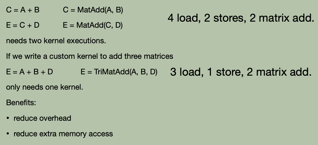
• 三个矩阵相加
  • 朴素实现：先计算 A+B 得到 C，然后计算 C+D 得到最终结果。
    • 需要两次 kernel launch。
    • 需要读显存 4 次，写 2 次。
  • Kernel Fusion：一个 kernel 完成 A+B+D。
    • 需要 1 次 kernel launch。
    • 减少了 1 次显存读和 1 次显存写。

1.1.1 Transformer Layer and Operator

MHA 与 FFN 层：

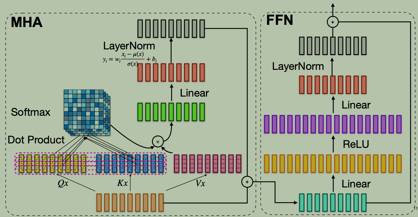
对应的算子（计算过程)：

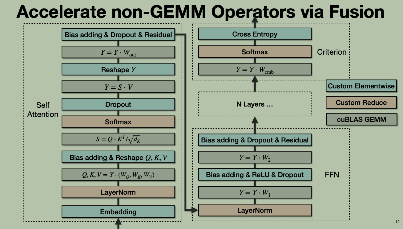
• 其中的非 GEMM op 可以通过 kernel fusion 加速。

1.1.2 Fused Embedding Operator

Forward

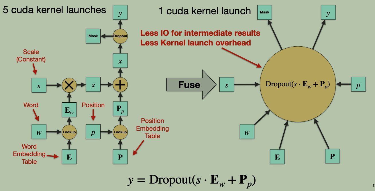
• Embedding 层 forward 计算过程
  • 朴素实现：需要 5 个 kernel
    • Word Embedding Lookup
    • Position Embedding Lookup
    • Word Embedding Scale
    • Word Embedding + Position Embedding
    • Dropout
  • Kernel Fusion：融合到 1 个 kernel 完成
    • \(y = \text{Dropout}\left(s \cdot \mathbf{E}_{w} + \mathbf{P}_{p}\right)\)

fwd fused kernel 代码：

• link: lightseq:embedding_kernels.cu

/**
 * @brief Fused Embedding Forward CUDA Kernel (词嵌入前向融合算子)
 * 
 * 融合操作包含：
 *   1. Token Embedding Lookup (词向量查找)
 *   2. Positional Embedding Lookup (位置向量查找)
 *   3. Token Scaling (词向量缩放, 如 sqrt(d_model))
 *   4. Fake Quantization (可选伪量化/截断)
 *   5. Dropout & Mask Saving (按元素 Dropout 并存掩码)
 *
 * =============================== 参数含义与 Shape 说明 ===============================
 * @param output          [输出] 融合计算后的词嵌入特征矩阵。
 *                        Shape: (batch_size, seq_len, embedding_dim) -> 展平 [B * S * D]
 *                        内部强转为 float4* 访问，内存按 128-bit (4 * float) 打包。
 * 
 * @param input           [输入] Token ID 矩阵 (Batch 内每个位置的词索引)。
 *                        Shape: (batch_size, seq_len) -> 展平 [B * S]
 * 
 * @param tokens_position [输入] 位置 Index 矩阵 (每个 Token 在序列中的位置 0~S-1)。
 *                        Shape: (batch_size, seq_len) -> 展平 [B * S]
 * 
 * @param embeddings      [输入] 词表嵌入矩阵 (Token Embedding Table)。
 *                        Shape: (vocab_size, embedding_dim) -> 展平 [V * D]
 * 
 * @param pos_embeddings  [输入] 位置嵌入矩阵 (Positional Embedding Table)。
 *                        Shape: (max_pos_len, embedding_dim) -> 展平 [P * D]
 * 
 * @param clip_max        [输入] 伪量化/截断阈值指针 (可选，不量化时传 nullptr)。
 *                        Shape: 标量指针 (1,) 或 nullptr
 * 
 * @param dropout_mask    [输出] 保存生成的 Dropout 掩码，供反向传播 (Backward) 复用。
 *                        Shape: (batch_size, seq_len, embedding_dim) -> 展平 [B * S * D]
 *                        内部强转为 uint32_t* 打包写入 (每 4 个 uint8_t 掩码打包为 1 个 uint32_t)。
 * 
 * @param seq_len         [输入] 序列长度 S (Sequence Length)。
 *                        Shape: 标量 (int)
 * 
 * @param embedding_dim   [输入] 词向量维度 D (Embedding Dimension)，通常需为 4 的倍数。
 *                        Shape: 标量 (int)
 * 
 * @param padding_idx     [输入] Padding 字符 ID (如 <pad>)，遇到该 ID 输出直接置 0。
 *                        Shape: 标量 (int)
 * 
 * @param dropout_ratio   [输入] Dropout 丢弃概率 (例如 0.1)。
 *                        Shape: 标量 (float)
 * 
 * @param emb_scale       [输入] 词向量缩放因子 (例如 Transformer 中的 sqrt(d_model))。
 *                        Shape: 标量 (float)
 * 
 * @param step            [输入] 自回归解码 (Inference) 时的当前步数偏移量 (训练阶段固定为 0)。
 *                        Shape: 标量 (int)
 * 
 * @param seed            [输入] CUDA 在卡 Philox 伪随机数生成器的随机种子。
 *                        Shape: 标量 (int)
 * ===================================================================================
 */
template <>
__global__ void lookup_scale_pos_dropout<float>(
    float *output, const int *input, const int *tokens_position,
    const float *embeddings, const float *pos_embeddings, const float *clip_max,
    uint8_t *dropout_mask, int seq_len, int embedding_dim, int padding_idx,
    float dropout_ratio, float emb_scale, int step, int seed) {
  // blockIdx.x 处理 batch 维度
  int batch_id = blockIdx.x;
  // blockIdx.y 结合 threadIdx.x/blockDim.x 确定 seq_id，处理 sequence 维度
  int seq_id = blockIdx.y * blockDim.x + threadIdx.x;
  if (seq_id >= seq_len) return;

  int target_pos = batch_id * seq_len + seq_id;
  // threadIdx.y 处理 embedding 维度
  int start = target_pos * embedding_dim + threadIdx.y;
  int end = (target_pos + 1) * embedding_dim;
  // token id, not thread id
  int tid = input[target_pos];

  int token_pos_id = tokens_position[target_pos];

  // 向量化访存
  float4 *output4 = reinterpret_cast<float4 *>(output);
  const float4 *embeddings4 = reinterpret_cast<const float4 *>(embeddings);
  const float4 *pos_embeddings4 =
      reinterpret_cast<const float4 *>(pos_embeddings);
  uint32_t *dropout_mask4 = reinterpret_cast<uint32_t *>(dropout_mask);

  // no need to calculate dropout_mask
  if (tid == padding_idx) {
    float4 zero4;
    zero4.x = zero4.y = zero4.z = zero4.w = 0.f;
    // 对于 padding token id，直接写回 0
    for (uint i = start; i < end; i += blockDim.y) {
      output4[i] = zero4;
    }
    return;
  }

  const float dropout_scale = 1.f / (1.f - dropout_ratio);
  float clip_max_val;
  if (clip_max) {
    clip_max_val = clip_max[0];
  }
  curandStatePhilox4_32_10_t state;

  for (uint i = start; i < end; i += blockDim.y) {
    curand_init(seed, i, 0, &state);
    float4 rand4 = curand_uniform4(&state);
    uint8_t m[4];
    // dropout mask
    m[0] = (uint8_t)(rand4.x > dropout_ratio);
    m[1] = (uint8_t)(rand4.y > dropout_ratio);
    m[2] = (uint8_t)(rand4.z > dropout_ratio);
    m[3] = (uint8_t)(rand4.w > dropout_ratio);

    int offset = i - target_pos * embedding_dim;
    // step is non-zero only in inference
    float4 e4 = embeddings4[tid * embedding_dim + offset];
    float4 pe4 =
        pos_embeddings4[(token_pos_id + step) * embedding_dim + offset];
    float4 res4;

    // apply dropout
    float scale_mask[4];
    scale_mask[0] = dropout_scale * m[0];
    scale_mask[1] = dropout_scale * m[1];
    scale_mask[2] = dropout_scale * m[2];
    scale_mask[3] = dropout_scale * m[3];

    uint8_t clip_mask[4];
    if (clip_max) {
      e4.x = fake_quantize(e4.x, clip_max_val, clip_mask[0], 2);
      e4.y = fake_quantize(e4.y, clip_max_val, clip_mask[1], 2);
      e4.z = fake_quantize(e4.z, clip_max_val, clip_mask[2], 2);
      e4.w = fake_quantize(e4.w, clip_max_val, clip_mask[3], 2);
    }
    // scale
    res4.x = (emb_scale * e4.x + pe4.x) * scale_mask[0];
    res4.y = (emb_scale * e4.y + pe4.y) * scale_mask[1];
    res4.z = (emb_scale * e4.z + pe4.z) * scale_mask[2];
    res4.w = (emb_scale * e4.w + pe4.w) * scale_mask[3];

    output4[i] = res4;
    uint32_t *m4 = reinterpret_cast<uint32_t *>(m);
    if (clip_max) {
      m4[0] = m4[0] | reinterpret_cast<uint32_t *>(clip_mask)[0];
    }
    dropout_mask4[i] = m4[0];
  }
}

Backward

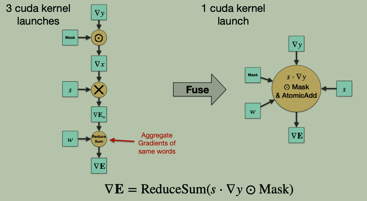
• Embedding 层 backward 计算过程
  • 朴素实现：3 个 kernel
    • Dropout backward：mask elementwise multiply，将上层传回的梯度 \(\nabla y\) 与前向传播保留的 Dropout Mask 进行元素级相乘 \(\nabla y \odot Mask\) 。
    • Scale backward：乘以相应的缩放因子 \(s\)，得到 \(s \cdot \nabla y \odot Mask\)。
    • Embedding Lookup backward：Reduce Sum，查找当前 Batch 中所有 Token 的 ID，对序列中多次出现相同词（Same Words）的梯度进行累加，最后写回词表梯度矩阵 \(\nabla E_w\)。
  • Kernel Fusion：1 个 kernel
    • \(\nabla \mathbf{E} = \text{ReduceSum}\left( s \cdot \nabla y \odot \text{Mask} \right)\)

backward fused kernel 代码：

• link: lightseq:embedding_kernels.cu

/**
 * @brief Fused Embedding Backward CUDA Kernel (词嵌入反向传播融合算子)
 *
 * 融合操作包含：
 *   1. Upstream Gradient Read (读取上层传回的梯度 grad_output)
 *   2. Dropout & Scale Backward (根据前向保存的 Mask 与 Scale 计算 Embedding 梯度)
 *   3. Fake Quantization Clip Backward (伪量化截断阈值的梯度计算)
 *   4. Embedding Gradient Accumulation (使用 atomicAdd 聚合 Batch 内相同词的梯度)
 *   5. Hierarchical Reduction for grad_clip_max (共享内存两级规约求截断阈值总梯度)
 *
 * =============================== 参数含义与 Shape 说明 ===============================
 * @param grad_embeddings [输出/累加] 词表嵌入矩阵的梯度 (Embedding Table Gradient)。
 *                        Shape: (vocab_size, embedding_dim_float) -> 展平 [V * D_float]
 *                        由于 Batch 内可能存在相同的词 ID，采用 atomicAdd 并发累加。
 *
 * @param grad_clip_max   [输出/累加] 伪量化截断阈值的梯度指针 (可选)。
 *                        Shape: 标量指针 (1,) 或 nullptr
 *
 * @param grad_output     [输入] 上层反向传播传回的梯度矩阵 (\nabla Y)。
 *                        Shape: (batch_size, seq_len, embedding_dim_float) -> 展平 [B * S * D_float]
 *                        内部强转为 const float4* 读取 (按 128-bit 打包)。
 *
 * @param input           [输入] Token ID 矩阵 (前向传入的输入词索引)。
 *                        Shape: (batch_size, seq_len) -> 展平 [B * S]
 *
 * @param dropout_mask    [输入] 前向传播时保存的 Dropout 掩码。
 *                        Shape: (batch_size, seq_len, embedding_dim_float) -> 展平 [B * S * D_float]
 *                        内部强转为 const uint32_t* 读取 (打包包含 4 个 uint8_t 掩码)。
 *
 * @param seq_len         [输入] 序列长度 S (Sequence Length)。
 *                        Shape: 标量 (int)
 *
 * @param embedding_dim   [输入] 向量化的词维度 (以 float4 为单位，即 D_float / 4)。
 *                        Shape: 标量 (int)
 *
 * @param padding_idx     [输入] Padding 字符 ID (如 <pad>)，遇到该 ID 跳过梯度计算。
 *                        Shape: 标量 (int)
 *
 * @param dropout_ratio   [输入] Dropout 丢弃概率 (例如 0.1)。
 *                        Shape: 标量 (float)
 *
 * @param emb_scale       [输入] 词向量缩放因子 (例如 Transformer 中的 sqrt(d_model))。
 *                        Shape: 标量 (float)
 * ===================================================================================
 */
template <>
__global__ void d_lookup_scale_pos_dropout<float>(
    float *grad_embeddings, float *grad_clip_max, const float *grad_output,
    const int *input, const uint8_t *dropout_mask, int seq_len,
    int embedding_dim, int padding_idx, float dropout_ratio, float emb_scale) {
  // 线程网格映射：确定 Batch 和 Sequence 维度位置
  int batch_id = blockIdx.x;
  int seq_id = blockIdx.y * blockDim.x + threadIdx.x;
  if (seq_id >= seq_len) return;

  // 计算全局 Token 索引与对应线程在 Embedding 维度的起始/结束偏移
  int target_pos = batch_id * seq_len + seq_id;
  int start = target_pos * embedding_dim + threadIdx.y;
  int end = (target_pos + 1) * embedding_dim;
  // token id
  int tid = input[target_pos];

  if (tid == padding_idx) {
    return;
  }

  const float scale = 1.f / (1.f - dropout_ratio);
  // 向量化读取
  const float4 *grad_output4 = reinterpret_cast<const float4 *>(grad_output);
  const uint32_t *dropout_mask4 =
      reinterpret_cast<const uint32_t *>(dropout_mask);
  // float block_g_clip_max = 0;
  float thread_cmax_grad = 0;
  float temp_cmax_grad = 0;
  // 沿 Embedding 维度迭代计算梯度（步长为 blockDim.y）
  for (uint i = start; i < end; i += blockDim.y) {
    float4 go4 = grad_output4[i];
    uint32_t m4 = dropout_mask4[i];
    uint8_t *m4_ptr = reinterpret_cast<uint8_t *>(&m4);
    float4 res4;
    // 链式法则：d_emb = emb_scale * grad_output * mask * scale
    res4.x = emb_scale * go4.x * (m4_ptr[0] & 1) * scale;
    res4.y = emb_scale * go4.y * (m4_ptr[1] & 1) * scale;
    res4.z = emb_scale * go4.z * (m4_ptr[2] & 1) * scale;
    res4.w = emb_scale * go4.w * (m4_ptr[3] & 1) * scale;
    int offset = i - target_pos * embedding_dim;
    int idx = (tid * (embedding_dim) + offset) << 2;
    clip_bwd(res4.x, temp_cmax_grad, res4.x, m4_ptr[0], 2);
    thread_cmax_grad += temp_cmax_grad;
    clip_bwd(res4.y, temp_cmax_grad, res4.y, m4_ptr[1], 2);
    thread_cmax_grad += temp_cmax_grad;
    clip_bwd(res4.z, temp_cmax_grad, res4.z, m4_ptr[2], 2);
    thread_cmax_grad += temp_cmax_grad;
    clip_bwd(res4.w, temp_cmax_grad, res4.w, m4_ptr[3], 2);
    thread_cmax_grad += temp_cmax_grad;
    // 使用 atomicAdd 原子加将梯度累加回全局词表梯度矩阵 grad_embeddings 
    // 原因：同一 Batch 或序列中可能出现多个相同的词 ID (tid)，并发写入会产生写冲突
    atomicAdd(grad_embeddings + idx, res4.x);
    atomicAdd(grad_embeddings + idx + 1, res4.y);
    atomicAdd(grad_embeddings + idx + 2, res4.z);
    atomicAdd(grad_embeddings + idx + 3, res4.w);
  }

  // grad_clip_max 的两级层次化规约 (Block Shared Memory -> Global Memory)
  if (grad_clip_max) {
    __shared__ float block_cmax_grad;
    if (threadIdx.x == 0 && threadIdx.y == 0) {
      block_cmax_grad = 0;
    }
    __syncthreads();
    if (thread_cmax_grad != 0) {
      atomicAdd(&block_cmax_grad, thread_cmax_grad);
    }
    __syncthreads();
    if (threadIdx.x == 0 && threadIdx.y == 0) {
      if (block_cmax_grad != 0) {
        atomicAdd(&grad_clip_max[0], block_cmax_grad);
      }
    }
  }
}

1.1.3 Gradient of Criterion Operator（CrossEntropyLoss）

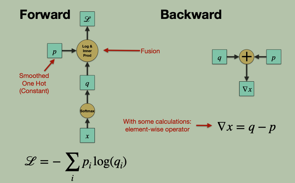
带 Label Smoothing 的 CrossEntropyLoss forward 流程：

• Label Smoothing 后目标概率分布 \(p\) ：

\[ p_i = (1 - \alpha) y_i + \frac{\alpha}{V} \]

其中 \(y_i\) 为原始的 One-hot 真实标签，\(\alpha\) 为标签平滑系数，\(V\) 为词表大小。

• 预测概率分布 \(q\) ：

\[ q_i = \text{Softmax}(x_i) = \frac{e^{x_i}}{\sum_j e^{x_j}} \] 其中 \(x\) 为 logits 向量。

• 交叉熵损失 \(\mathcal{L}\)：

\[ \mathcal{L} = -\sum_i p_i \log(q_i) \]

• 朴素实现：
  • Label Smoothing
  • Softmax
  • log
  • 向量内积
• Kernel Fusion：
  • 输入 Logits \(x\) 和标签 \(y\)，一步到位输出 Loss \(\mathcal{L}\) 和预测概率 \(q\)

反向传播 Fusion 推导：

通过对损失函数 \(\mathcal{L}\) 直接推导关于输入 Logits \(x_k\) 的偏导数（利用 \(\sum_i p_i = 1\) 的性质，Softmax 梯度的分母项与交叉熵求导项相互抵消）：

\[ \nabla_x \mathcal{L} = \frac{\partial \mathcal{L}}{\partial x} = q - p \]

具体推导过程如下：

• Softmax 导数：

\[ \frac{\partial \mathbf{q}_i}{\partial \mathbf{h}_j} = \begin{cases} \mathbf{q}_i (1 - \mathbf{q}_i), & \text{if } i = j \\ -\mathbf{q}_i \mathbf{q}_j, & \text{if } i \neq j \end{cases} \]

• 损失函数对 Logit \(\mathbf{h}_i\) 求导：

根据链式法则：

\[ \nabla \mathbf{h}_i = \frac{\partial \mathcal{L}}{\partial \mathbf{h}_i} = -\sum_j \frac{\mathbf{p}_j}{\mathbf{q}_j} \cdot \frac{\partial \mathbf{q}_j}{\partial \mathbf{h}_i} \]

按目标位置 \(i\) 是否为 Ground Truth 分情况讨论：

1) 当 \(i = k\) （即 Token \(i\) 是真实标签）时：

\[ \begin{aligned} \nabla \mathbf{h}_k = \frac{\partial \mathcal{L}}{\partial \mathbf{h}_k} &= -\frac{\alpha}{V} \sum_{j \neq k} \frac{1}{\mathbf{q}_j} \cdot \frac{\partial \mathbf{q}_j}{\partial \mathbf{h}_k} - \left(1 - \alpha + \frac{\alpha}{V}\right) \cdot \frac{1}{\mathbf{q}_k} \cdot \frac{\partial \mathbf{q}_k}{\partial \mathbf{h}_k} \\ &= -\frac{\alpha}{V} \sum_{j \neq k} \frac{1}{\mathbf{q}_j} (-\mathbf{q}_j \mathbf{q}_k) - \left(1 - \alpha + \frac{\alpha}{V}\right) \cdot \frac{1}{\mathbf{q}_k} \cdot \mathbf{q}_k (1 - \mathbf{q}_k) \\ &= \frac{\alpha}{V} \sum_{j \neq k} \mathbf{q}_k - \left(1 - \alpha + \frac{\alpha}{V}\right) (1 - \mathbf{q}_k) \\ &= \frac{\alpha}{V} (V - 1) \mathbf{q}_k - \left(1 - \alpha + \frac{\alpha}{V}\right) (1 - \mathbf{q}_k) \\ &= \mathbf{q}_k - \frac{\alpha}{V} - 1 + \alpha \end{aligned} \]

2) 当 \(i \neq k\) （非真实标签位置）时： \[ \begin{aligned} \nabla \mathbf{h}_i = \frac{\partial \mathcal{L}}{\partial \mathbf{h}_i} &= -\frac{\alpha}{V} \sum_{j \neq k, j \neq i} \frac{1}{\mathbf{q}_j} \cdot \frac{\partial \mathbf{q}_j}{\partial \mathbf{h}_i} - \frac{\alpha}{V} \cdot \frac{1}{\mathbf{q}_i} \cdot \frac{\partial \mathbf{q}_i}{\partial \mathbf{h}_i} - \left(1 - \alpha + \frac{\alpha}{V}\right) \cdot \frac{1}{\mathbf{q}_k} \cdot \frac{\partial \mathbf{q}_k}{\partial \mathbf{h}_i} \\ &= -\frac{\alpha}{V} \sum_{j \neq k, j \neq i} \frac{1}{\mathbf{q}_j} (-\mathbf{q}_j \mathbf{q}_i) - \frac{\alpha}{V} \cdot \frac{1}{\mathbf{q}_i} \cdot \mathbf{q}_i (1 - \mathbf{q}_i) - \left(1 - \alpha + \frac{\alpha}{V}\right) \cdot \frac{1}{\mathbf{q}_k} (-\mathbf{q}_k \mathbf{q}_i) \\ &= \frac{\alpha}{V} \sum_{j \neq k, j \neq i} \mathbf{q}_i - \frac{\alpha}{V} (1 - \mathbf{q}_i) + \left(1 - \alpha + \frac{\alpha}{V}\right) \mathbf{q}_i \\ &= \mathbf{q}_i - \frac{\alpha}{V} \end{aligned} \]

整理上述两项，对任意分量 \(i\) 的梯度表达为： \[ \nabla \mathbf{h}_i = \begin{cases} \mathbf{q}_i - \frac{\alpha}{V} - 1 + \alpha, & \text{if token } i \text{ is the ground truth} \\ \mathbf{q}_i - \frac{\alpha}{V}, & \text{otherwise} \end{cases} \]

结合前面定义的真实分布 \(\mathbf{p}_i\)，上式可以精简并统一表示为向量级别的逐元素减法： \[ \mathbf{g} = \nabla_{\mathbf{h}} \mathcal{L} = \mathbf{q} - \mathbf{p} \]

Fused Criterion Operator 示意图：

1.1.4 Layer-Batched Cross Attention

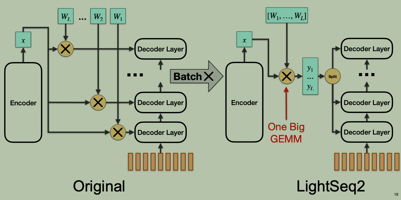
将原本 encoder 输出特征与 \(L\) 层 decoder 权重计算得到 \(L\) 个 Key/Value（\(L\) 次 kernel launch），fuse 成一个 kernel 完成 \(L\) 层的所有 Key 或者 Value 计算，即将多个小的 GEMM 融合为一个大 GEMM。示意图：

1.2 Reduce synchronization

1.2.1 Rewrite Reduction: LayerNorm

forward

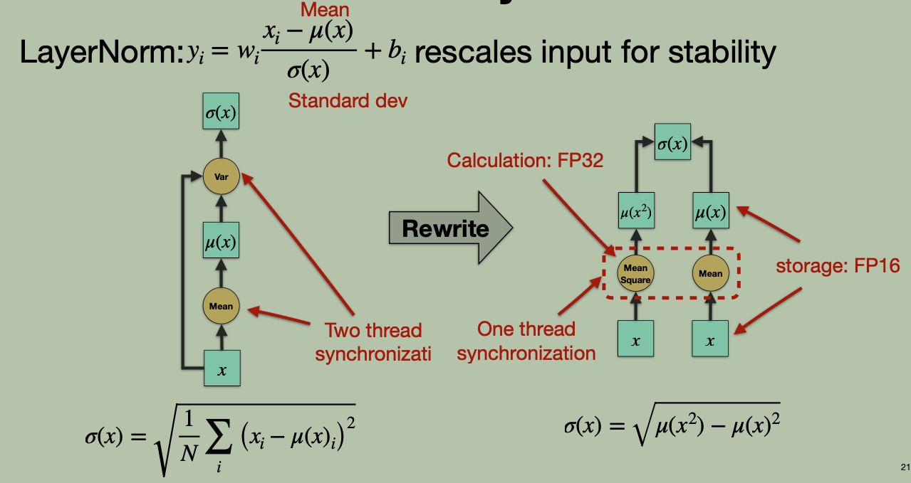
• 朴素实现方式：
  • 先计算均值，再基于均值计算标准差。
  • 需要两次 kernel 内同步。
• 改进实现方式：
  • 利用公式 \(\sigma(x) = \sqrt{\mu(x^2) - {\mu(x)}^2 }\) ，即：标准差/方差等于“平方的均值”减去“均值的平方”。
  • 线程在同一趟遍历中，可以同时并行累加 \(x_i\) 的和以及 \(x_i^2\) 的和，一次性同时求出均值 \(\mu(x)\) 和平方均值 \(\mu(x^2)\)。只需要一次 kernel 内同步。
  • 数值精度：存储采用 FP16，而内部累加计算采用 FP32 以保证精度。

backward

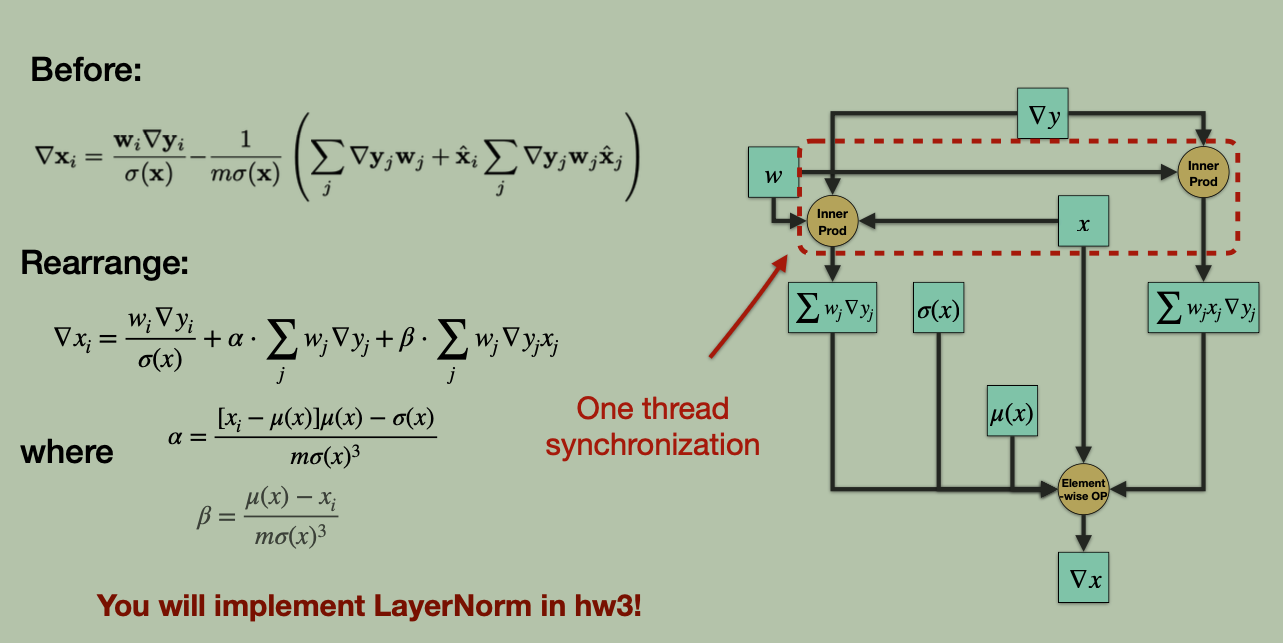
符号含义说明：

• \(\mathbf{x}\) 与 \(x_i\)（输入特征）：
  • \(\mathbf{x}\)：LayerNorm 的输入特征向量（如一个 Token 的隐藏层向量）。
  • \(x_i\)：输入向量中第 \(i\) 个通道/维度上的具体数值（\(i = 1, 2, \dots, m\)）。
  • \(x_j\)：求和公式中用于遍历所有通道的下标符号。
• \(\mathbf{y}\) 与 \(y_i\)（输出特征）：
  • \(\mathbf{y}\)：LayerNorm 归一化并缩放平移后的输出特征向量。
  • \(y_i\)：输出向量中第 \(i\) 个维度的具体数值。
• \(m\)（特征维度大小）：
  • 隐藏层向量的总维度/通道数（Hidden Dimension Size，即向量 \(\mathbf{x}\) 里一共有多少个元素）。在求均值和方差时作为分母除数 \(\frac{1}{m}\)。
• \(i, j\)（通道下标索引 Index）：
  • \(i\) 代表我们当前正在计算的那个特定通道。
  • \(j\) 代表在做全局求和（\(\sum_j\)）时遍历的所有通道（从 \(1\) 到 \(m\)）。
• \(w_i\)（缩放权重 Weight / Gamma \(\gamma\)）：
  • 模型可学习的缩放系数，用来恢复模型的表达能力。\(w_i\) 是第 \(i\) 个通道专属的权重。
• \(b_i\)（平移偏置 Bias / Beta \(\beta_{\text{bias}}\)）：
  • 模型可学习的偏移量。\(b_i\) 是第 \(i\) 个通道专属的偏置。
• \(\mu(\mathbf{x})\)（均值 Mean）：
  • 输入向量 \(\mathbf{x}\) 在所有通道上的平均值：\(\mu(\mathbf{x}) = \frac{1}{m} \sum_{k=1}^m x_k\)。
• \(\sigma(\mathbf{x})\)（标准差 Standard Deviation）：
  • 输入向量 \(\mathbf{x}\) 在所有通道上的标准差：\(\sigma(\mathbf{x}) = \sqrt{\frac{1}{m} \sum_{k=1}^m (x_k - \mu(\mathbf{x}))^2}\)。
• \(\sigma(\mathbf{x})^2\)（方差 Variance）：
  • 标准差的平方，即输入的方差。
• \(\hat{\mathbf{x}}_i\)（归一化后的临时特征）：
  • 零均值、单位方差的标准特征：\(\hat{\mathbf{x}}_i = \frac{x_i - \mu(\mathbf{x})}{\sigma(\mathbf{x})}\)。
• \(\nabla y_i\) 或 \(\nabla \mathbf{y}_i\)（上层传回的梯度）：
  • 损失函数 \(\mathcal{L}\) 对 LayerNorm 输出 \(y_i\) 的偏导数 \(\frac{\partial \mathcal{L}}{\partial y_i}\)（由网络后续层反向传回）。
• \(\nabla x_i\) 或 \(\nabla \mathbf{x}_i\)（需要求解的梯度）：
  • 损失函数 \(\mathcal{L}\) 对 LayerNorm 输入 \(x_i\) 的偏导数 \(\frac{\partial \mathcal{L}}{\partial x_i}\)（求出后继续向前传递给上一层）。
• 原始形式：
  • 第二项 sum 依赖于 mean/std，需要两次同步。
• 变换后形式：
  • 第二项 sum 依赖于输入，只需要一次同步。

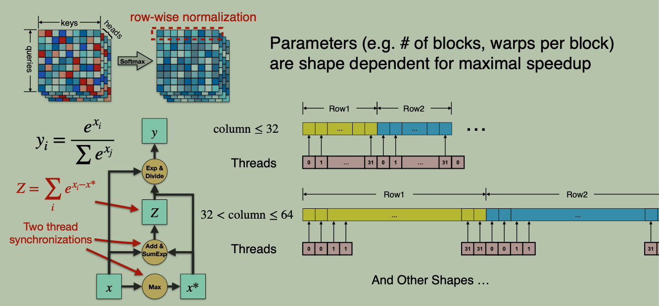
1.2.2 Rewrite Reduction: Softmax Forward

传统 Safe Softmax 的计算痛点（3 趟遍历 + 2 次同步）

为了防止浮点数指数运算 \(e^{x_i}\) 发生 overflow，实际工程中必须使用数值安全的 Safe Softmax： \[ y_i = \text{Softmax}(x_i) = \frac{e^{x_i - m}}{\sum_{j=1}^N e^{x_j - m}} \quad \text{其中 } m = \max_{j} x_j \]

在未优化的传统实现中，这一过程需要 3 趟数据遍历（3 Passes） 和 2 次线程同步屏障：

1. Pass 1 (Max Reduction)：遍历整行元素，找到最大值 \(m = \max(x_j)\)。此时需要 第 1 次线程同步，等待所有线程拿到全局最大值 \(m\)。
2. Pass 2 (SumExp Reduction)：再次遍历整行，计算减去最大值后的指数和 \(S = \sum e^{x_j - m}\)。此时需要 第 2 次线程同步，等待所有线程拿到全局和 \(S\)。
3. Pass 3 (Element-wise Division)：第三次遍历，计算最终归一化结果 \(y_i = \frac{e^{x_i - m}}{S}\)。

优化实现：

• Parameters (e.g. # of blocks, warps per block) are shape dependent for maximal speedup.
• 根据 dim 大小进行不同 kernel template 特化，以加速计算过程。

1.3 Mixed-precision Calculation

• Modern GPU supports half-precision (FP16) or FP8 (on H100)
• Benefits
  • lower memory for storing model and data ==> enlarge batch size.
  • transfer data at a higher rate (with same bandwith) between GPU main memory and SMs.
  • more FLOPs for FP16 (up to 8x more) compared to FP32.

低精度适用范围：

• Forward / Backward could use FP16 or FP8.
• Gradient update in Optimizer (or trainer) needs FP32.
• Nvidia APEX library provides automatic mixed-precision calculation for many NN layers.
  • but still miss fine-grained memory optimization with mixed-precision for LLM.

Accelerated Mixed-Precision Update

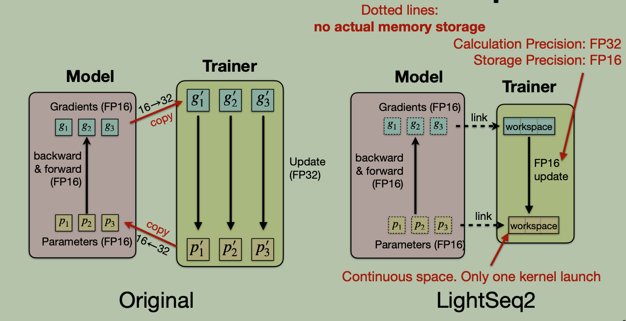
• 朴素实现：
  • 需要在显存中额外维护一份完整 FP32 浓度的 主权重（Master Weights）与主梯度。更新时需要将 FP16 参数与梯度复制成 FP32，用 FP32 更新完主权重后，再复制回 FP16。
  • 频繁的 Kernel Launch 与内存搬运：传统实现中，模型每个层/张量（Tensor）都是独立分散存放的，每次参数更新会为每个张量单独启动一次 CUDA Kernel，导致产生上百/上千次内核启动与昂贵的显存复制（Memory Copy）开销。
• LightSeq2：
  • 存储层面：显存中仅保持 FP16 的参数和梯度。
  • 计算层面：在 GPU 寄存器内部以 FP32 精度进行高精度的累加与更新计算。
  • 连续内存空间 (Continuous Space) 将模型所有层的 FP16 参数和梯度平铺映射到一段 连续的内存空间（Workspace） 中，取代原先分散独立的张量内存布局。
  • 单个内核一次性更新 (Only One Kernel Launch) 由于所有的参数和梯度都在连续内存空间中，整个 Optimizer 参数更新过程不再逐张量 Launch，而是全局仅发起 1 次 CUDA Kernel Launch，完成全模型所有参数的更新。
  • 消除显存实体备份 (Dotted lines: no actual memory storage) 上图中的虚线框表示 没有实际的 FP32 主权重/主梯度显存实体。Kernel 在读取 FP16 数据后，在寄存器中直接转换为 FP32 完成更新，并直接写回 FP16 显存中，消除了 FP32 内存实体的占用。

1.4 Memory Reuse

GPU Memory Management for Self Attention Backward

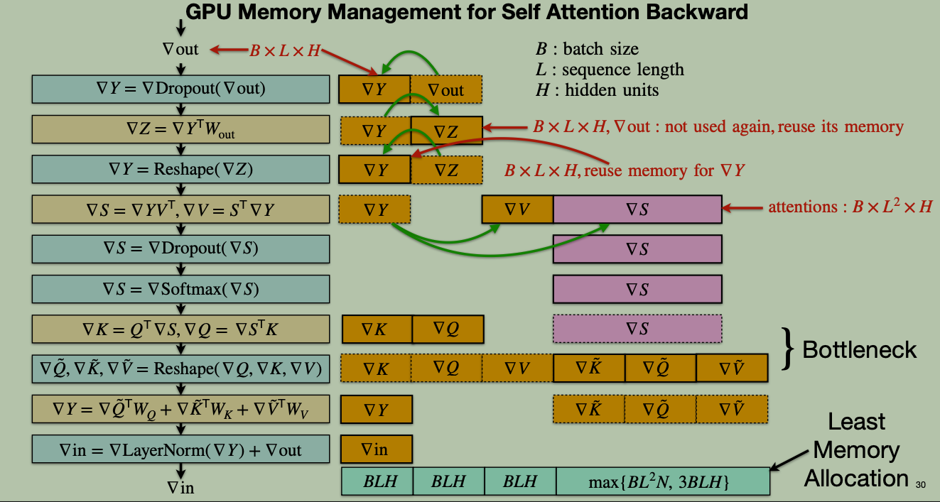
• backward 计算时
  • 识别出生命周期结束的张量。
  • 将后创的梯度张量直接写入原张量的显存地址中。
  • 大幅减少了训练阶段反向传播的显存峰值，使得 GPU 能够容纳更大的 Batch Size 或更长的输入序列 \(L\)。

1.5 Summary

• High performance Kernels for Forward and Backward
• Efficient Parameter Update
• Memory Management: Reuse Memory

key techniques

• Kernel Fusion: merge kernels other than matmul
• Algebraic Transformation: reduce sync
• Mix-precision calculation (use half precision whenever possible)
• Memory reuse (dependent on architecture)

2. Fast Inference for Transformer

2.1 Hierarchical Auto Regressive Search (HARS) for decoding

Beam Search 存在的问题

在传统的 Beam Search 解码中，每一步生成都需要：

1. 计算当前 Beam 中所有候选词的条件概率分布（Softmax）。
2. 计算累计序列概率，并在全局的 \(k \times V\) 个候选元素中选出得分最高的前 \(k\) 个序列（Top-\(k\)）。
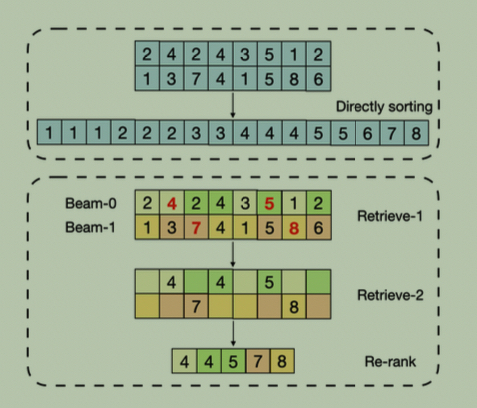
3. 存在的问题：当词表 \(V\) 很大（如 30,000+）时，直接对 \(k \times V\) 个元素进行全局排序（Direct Sorting）会在 GPU 上引发巨大的显存访存开销与线程同步等待。

HARS 的核心思想

HARS 的核心优化策略是 “先粗筛过滤，再局部精排” （retrieve and re-rank）：

• 不再直接对全部 \(k \times V\) 个元素执行昂贵的全局 Top-\(k\) 排序。
• 将大规约排序拆解为 并行 Max 过滤（Retrieve） 与 小规模候选重排（Re-rank），减少最终需要参与排序的元素数量。

算法流程：

第一步：检索阶段 (Retrieve Step)

1. 分组 (Divide Groups)：将每个 Beam 的 \(V\) 个 Logit 划分为 \(G\) 个小组。
2. 组内求最大值 (Group Maximums)：计算每个小组内的最大值，记为 \(m_i\)。
3. 求阈值 (Rough Lower Bound)：求当前 Beam 中所有小组最大值 \(m_i\) 中的最小值，记作粗略截断阈值 \(m_{\min}\)。
4. 粗筛过滤 (Filter)：只筛选出大于 \(m_{\min}\) 的 Logit，并写入 GPU 候选内存中，丢弃大部分极低概率的词。

第二步：重排阶段 (Re-rank Step)

• 对粗筛后保留下来的少数字候选 Logit 执行最终的 Top-\(k\) 排序（Re-rank）。

2.2 Details in GPU Inference Implementation

• share tensor memory across layers
• mixed precision computation, mostly using FP16 for computation
• Using float4 and half2 to increase bandwidth
• No need to keep intermediate results and gradients during infernece, similar to with torch.no_grad()

2.2 Summary

Accelerating decoding

• hierarchical auto-regressive search for large vocabulary
  • converting sorting to parallel operations (max, filter, re-rank)

Other Approaches for Acceleration

• Alternative Model Structures: Linformer, Reformer
• Training Strategy: Shallow to Deep, Layer Dropout
• Efficient Computation: LAMB, Quantization, Hardware Optimization